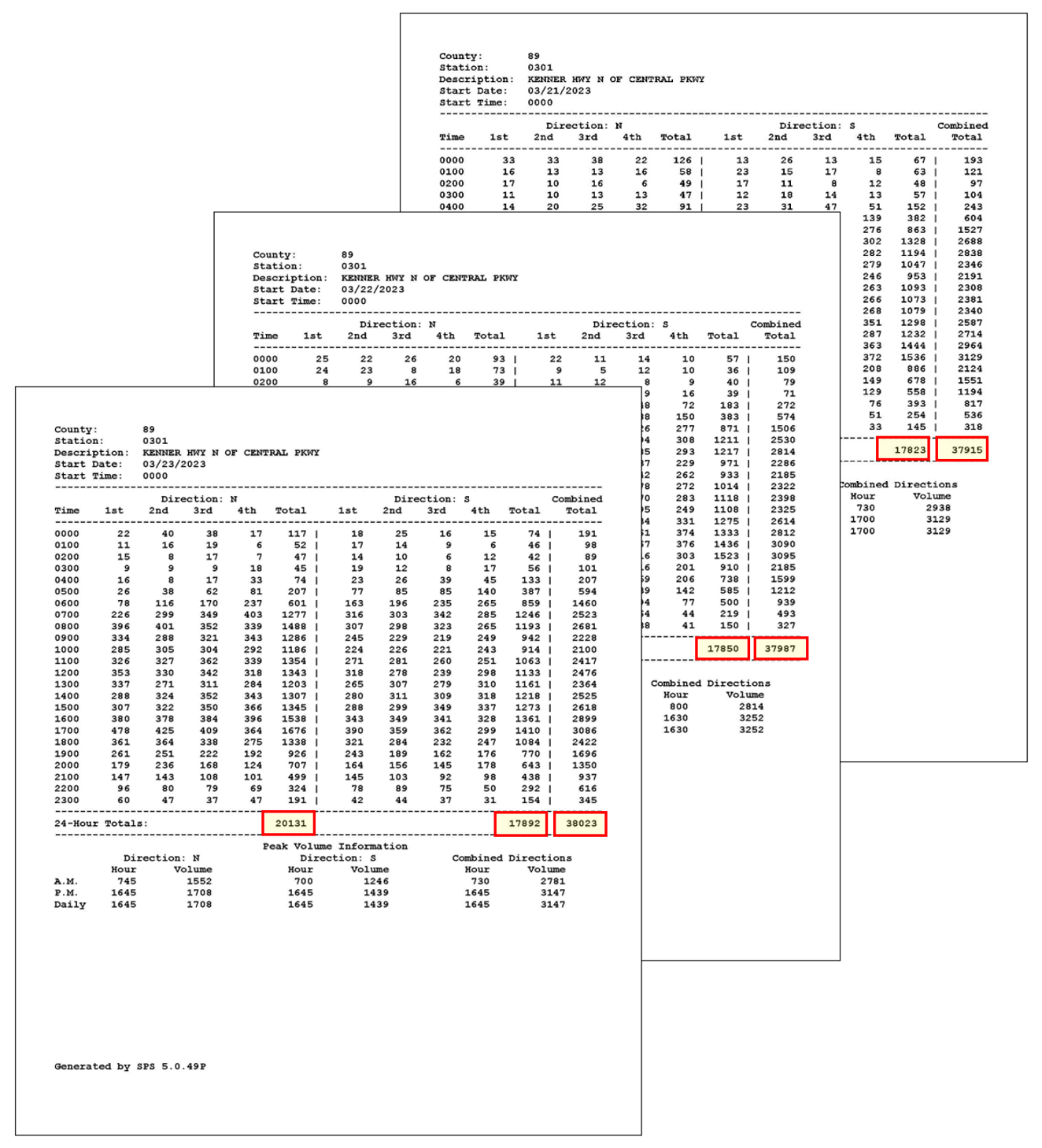
The following steps illustrate the process to estimate AADT from short-term traffic counts conducted along a highway section. In this example, three-day 72-hour traffic counts were taken by portable axle counters on Kenner Highway approximately 550 feet north of Central Parkway from Tuesday, 3/21/2023 to Thursday, 3/23/2023 in Martin County.

Step 1: Review Traffic Counts for Consistency and Reasonableness

Figure 1-1 shows the 3-day short-term traffic counts collected on Kenner Highway. The directional counts and the total daily counts collected for the three weekdays are consistent. Hourly volumes for the three days also show a similar pattern. Therefore, traffic counts from all three days will be used to calculate the ADT.

ADT= (37,915+37,987+38,023)/3=37,975

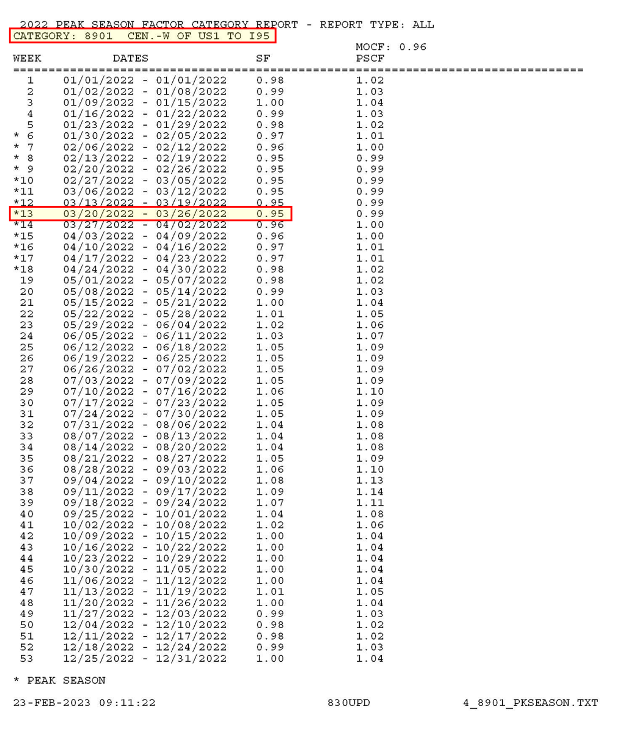
Step 2: Assign a Seasonal Factor from the Peak Season Factor Category Report

There are four volume factor categories for Martin County, three for the different geographic areas of the county, and one for I-95:

• Category: 8901 CEN.-W OF US1 TO I-95
• Category: 8900 EAST- A1A TO US1
• Category: 8927 WEST-W OF I-95
• Category: 8995 MARTIN I-95

The short-term traffic counts were collected in Central Martin County between West of US 1 and I-95, an area covered by Category 8901. Therefore, the seasonal factor from Category 8901 corresponding to the week of 03/20/2022 - 03/26/2022 was assigned to this location and the value of SF is 0.95 (See Figure 1-2).

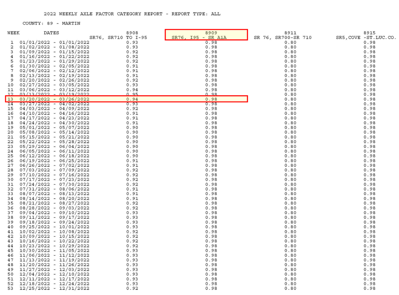
Step 3: Assign an Axle Correction Factor (ACF) from the Weekly Axle Correction Factor Category Report

Similar to Seasonal Factors, the ACF is obtained from the Weekly Axle Correction Factor Category Report. The ACFs are reported by facility, segment, and week. For roadways that do not belong to any of the included facility categories, the ACF for countywide rural, countywide urban, or countywide category can be used. There are 17 ACF categories for Martin County. The category that is most suitable for Kenner Highway is Category 8909 - SR76, I95 - SR A1A. The ACF for Category 8909 corresponding to the week of 03/20/2023 - 03/26/2022 is 0.98 (See Figure 1-3).

Step 4: Estimating AADT by Applying Adjustment Factors

AADT=ADT×SF×ACF

AADT=37,975×0.95×0.98=35,345

AADT=35,500 (After applying Rounding)

The following steps illustrate the process to develop project traffic for a road widening project in Columbia County. Columbia County is not currently covered by any of the regional models in Florida. To forecast future year traffic for roadways in Columbia County, trend projection procedures will be used. This example also serves as a demonstration of the use of the FDOT Trend Analysis Tool

Step 1: Assemble Available Data

1) Project Location Map

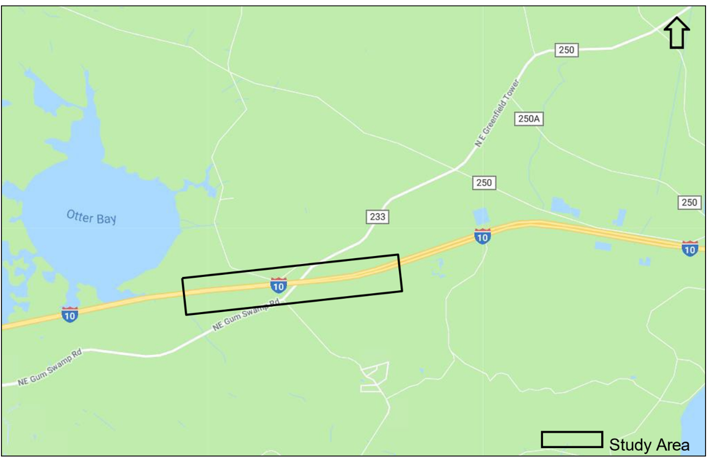
In this example, the project is located on I-10/SR-8 near CR-250 Overpass in Columbia County. It currently has two lanes in each direction. The project requires Year 2045 AADT at this location to determine the number of lanes needed in the future. Figure 2-1 shows the project location.

2) Historical Traffic Counts

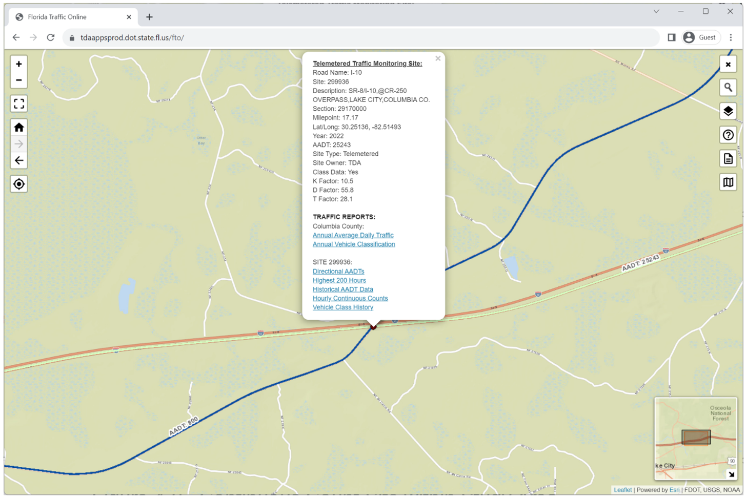
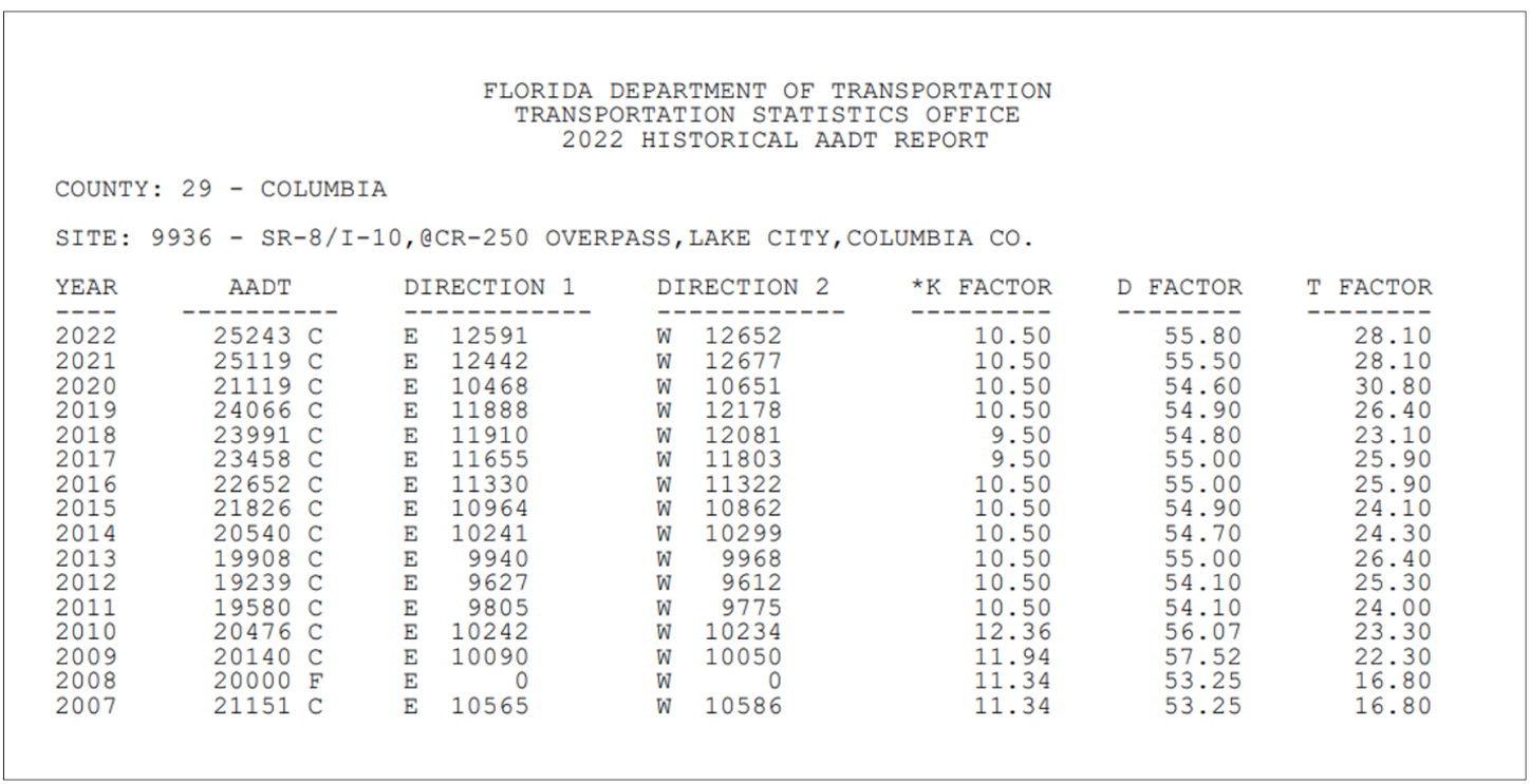
Based on Florida Traffic Online, Continuous TMS 299936 is located within the study area, and historical traffic counts are available from 2007 to 2022. (See Figure 2-2 and Figure 2-3).

3) Historical Population Data

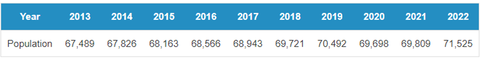
The Bureau of Economic and Business Research (BEBR) publishes annual population estimates by county by district on their websites. Historical population data can be obtained from these sources. Table 2-1 shows the historical population for Columbia County for the ten years from 2013 to 2022.

Table 2-1 Historical Population Estimates for Columbia County

4) FDOT Population Projections from 2025 to 2045

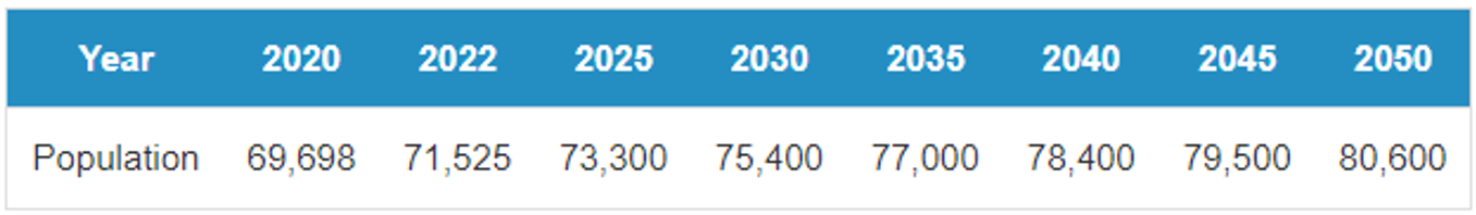
FTO publishes population projections by county. The most recent available data is for Years 2020 to 2045 in five- year increment adjusted based on 2022 population estimates. Table 2-2 shows the population for Columbia County for Census Year 2020, Year 2022, and projections for the years 2025 to 2050.

Table 2-2 - FDOT Population Projections for Columbia County

Step 2: Conduct Regression Analysis using Historical Traffic Data

The Traffic Trends Analysis Tool is a macro-based spreadsheet application developed by FDOT to perform historical trend analysis from specified FDOT sites or user defined locations. This Excel spreadsheet includes tabs of Instructions, Main Menu, Output, and Summary. The steps for trends analysis are described as follows:

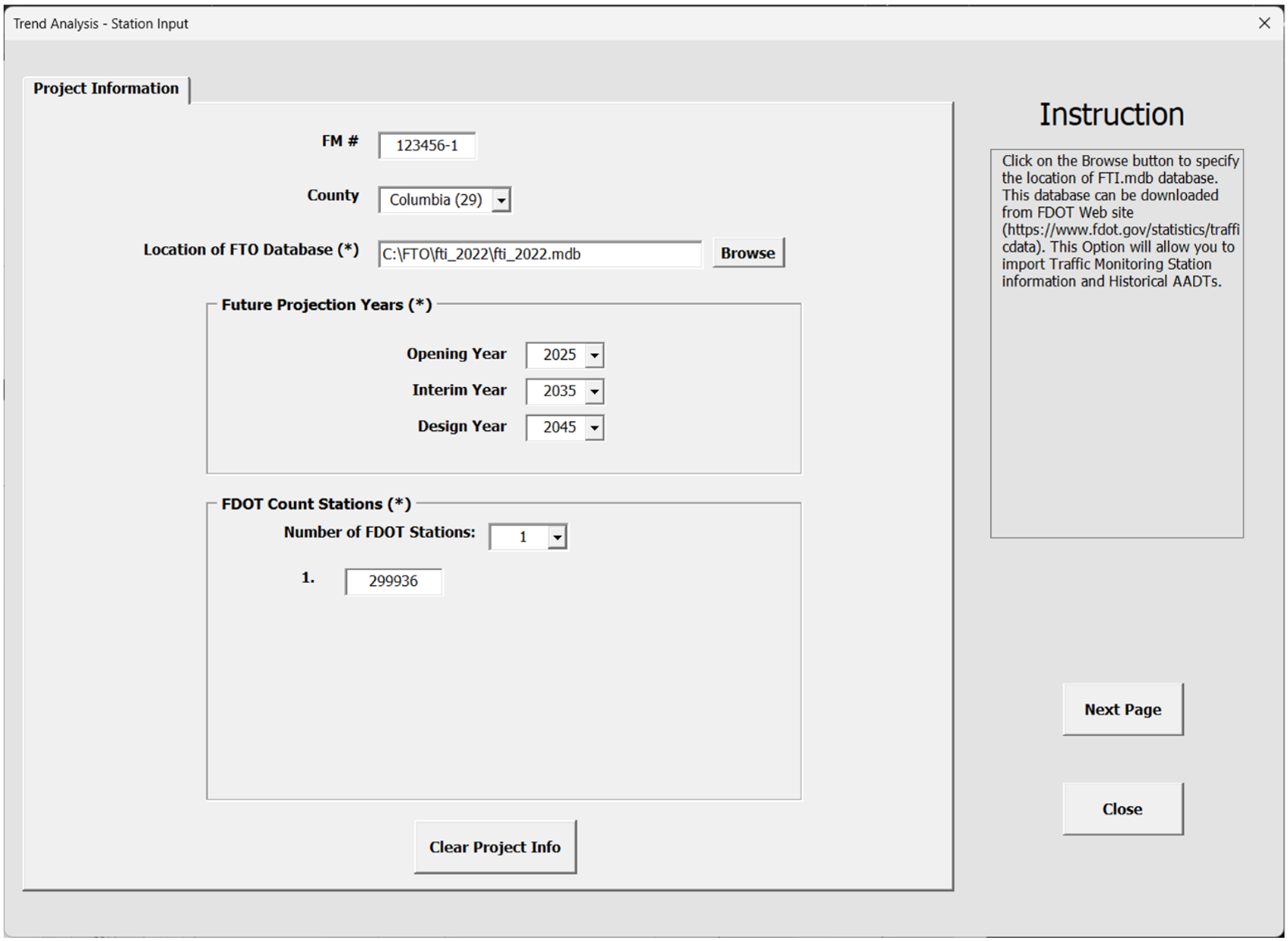
1. Open Main Menu and click Data Input, then enter Project Information. The project information includes FM number, County, location of the Florida Traffic Online (FTO) Database. Future projection years include opening year, interim year, and design year. Up to 10 FDOT count stations can be analyzed at one time. FDOT count station numbers need to be entered. Figure 2-4 shows the Project Information screen for Count Station 299936.

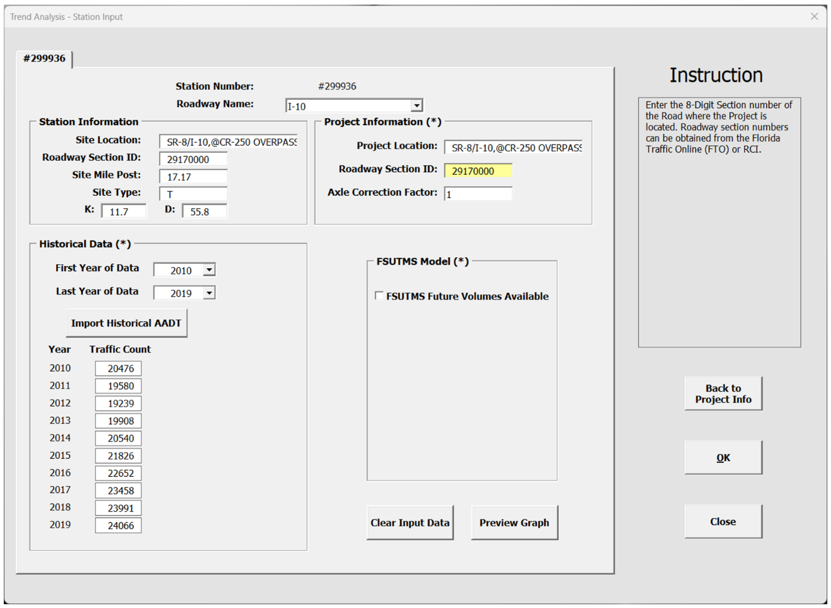
2. Enter Station Information. The station information will be automatically filled in if the FDOT count station is specified. Once the first year and last year of AADT volumes are specified, click on the "Import Historical AADT" button to load the historical AADTs from first year to last year from the FTO database. In this example, a typical 10-year AADT dataset from 2010 to 2019 was used. More recent data from 2020 to 2022 was not used because a careful examination of the data determined that those data were still under an impact of COVID 19. Figure 2-5 shows the Input Data screen for Site 299936.

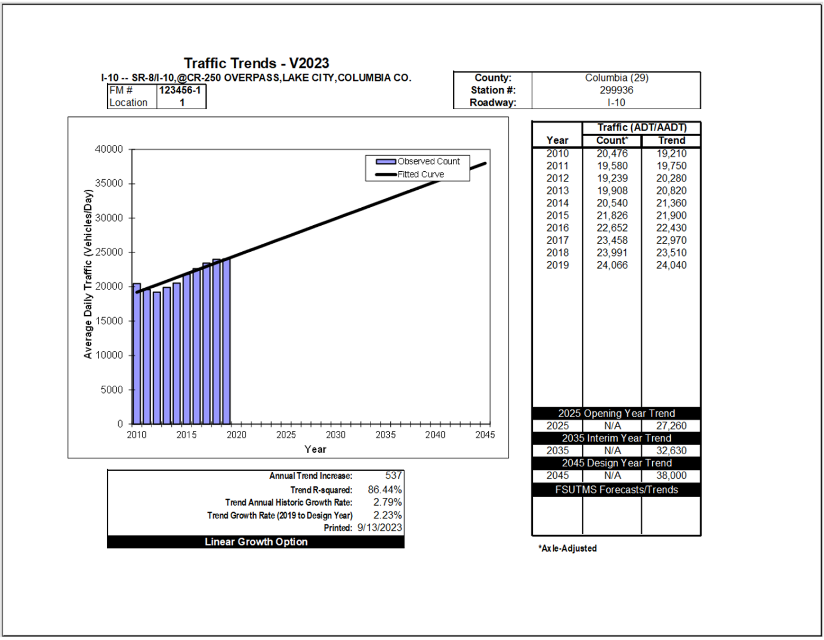
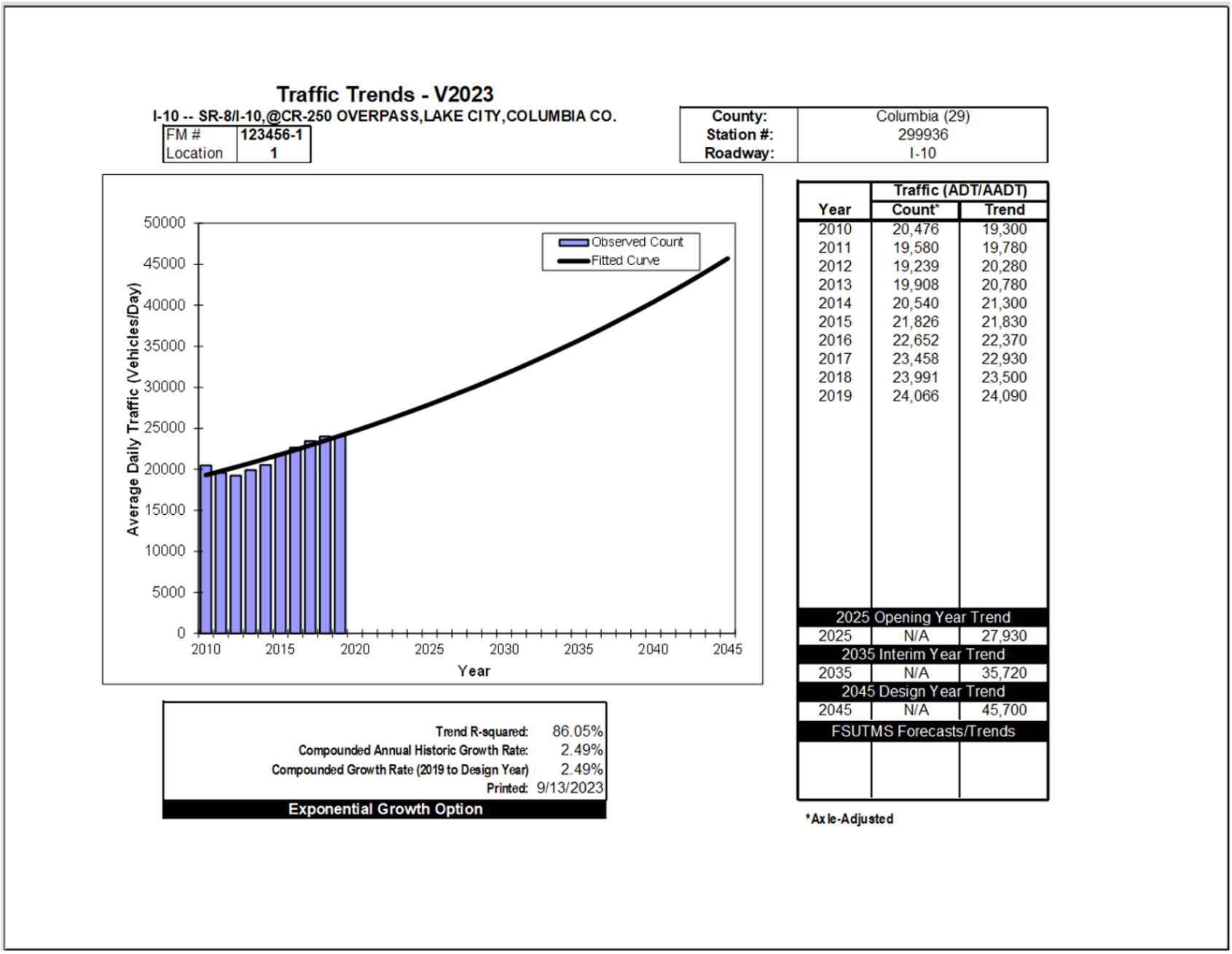
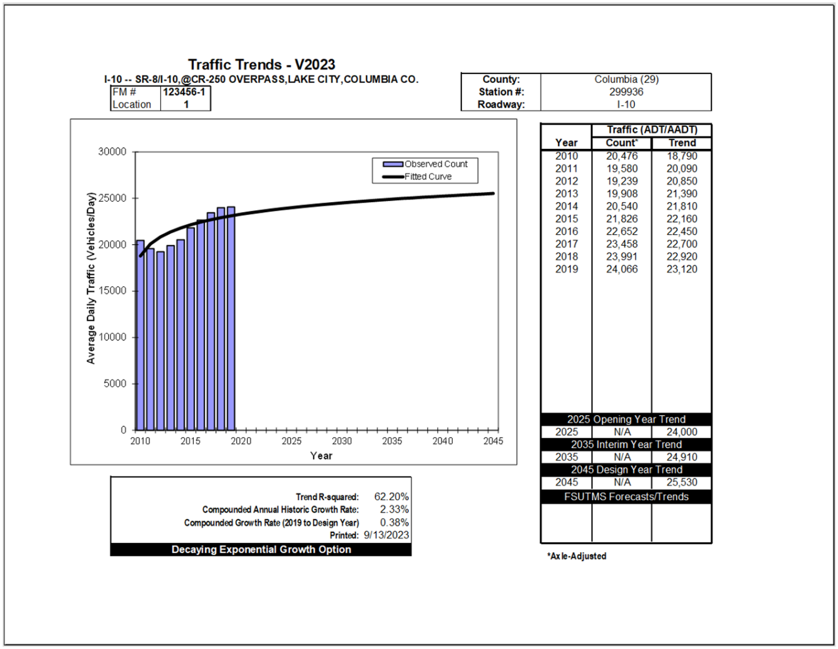
3. Once the historical data is imported or typed in, click on the "Preview Graph" Button to preview the trends analysis graphs using Linear, Exponential, and Decaying Exponential methods. Figures 2-6 to 2-8 show an example of three trends analysis graphs for the FDOT count station 299936.

4. Print results. Click on the "Print" button to print the trend analysis graphs for all the sites at one time.

5. View Results summary: open Main Menu and click "Analysis Summary" button to show the summary of the trend analysis results for all the sites. Table 2-3 shows the analysis summary for Site 299936.

Table 2-3 - FDOT Population Projections for Columbia County

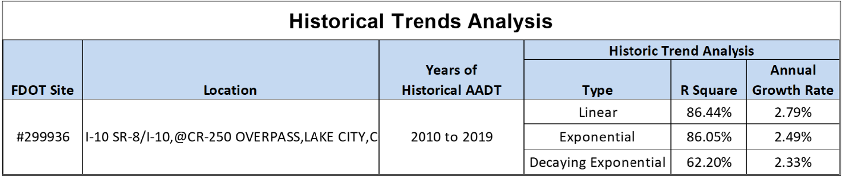
From the analysis summary, Linear Growth shows the highest R-Squared value of 86.44%, indicating a high correlation between AADT and the years. The annual growth rate is determined to be 2.79%.

Step 3: Review Traffic Projections for Reasonableness

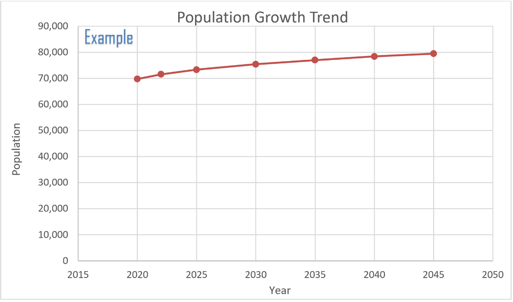
According to FDOT’s Population Projections from 2020 to 2045, the population of Columbia County is expected to increase from 69,698 in 2020 to 79,500 in 2045 (See Figure 2-9). This is an average of 0.56% in linear growth per year.

A comparison was then made to historical population data. Using BEBR population estimates, Columbia County’s population increased from 67,489 in 2013 to 71,525 in 2022. This was a 6.0% increase over a 10-year period, or an average of 0.60% in linear growth per year. By comparison, traffic increased from 20,476 in 2010 to 24,466 in 2019. This is a 17.5 % linear increase over a 10-year period, or an average of 1.75% in linear growth year. Therefore, it is apparent that the trend forecast showing future traffic increasing at a rate higher than the rate of population growth is consistent with the past trend over the last 10 years.

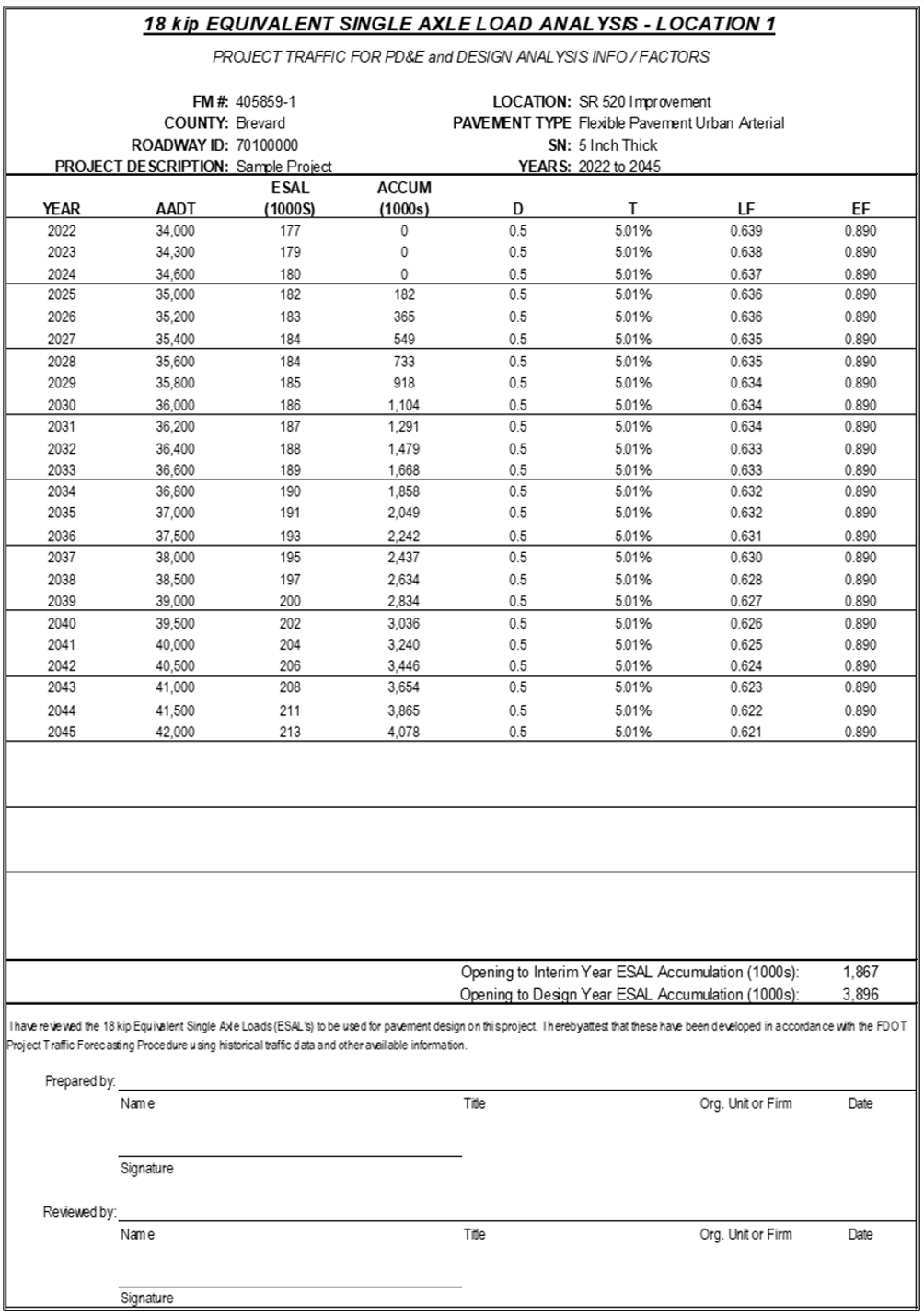
The following steps illustrate the process to generate the 18-KIP ESAL and the use of the FDOT ESAL Tool.

Step 1: Receive Request for 18-KIP ESAL Estimation

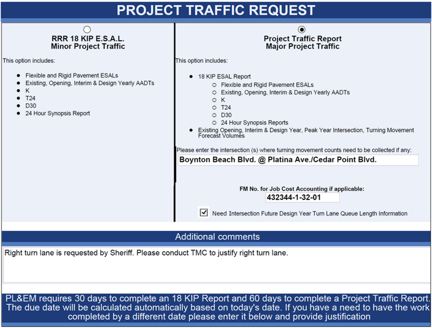
Figure 3-1 shows an example of Project Traffic Request form. Typical information requested includes AADT for project analysis years, K, D, and T factors, turning movement volumes, and 18-KIP ESAL Report.

Step 2: Collect Traffic and Geometric Information about the Facility

Additional information including Functional Classification (RCI Feature 121), Through Lanes (RCI Feature 212), Median (RCI Feature 215), Speed Limits (RCI Feature 311) and Traffic Flow Breaks (RCI Feature 331) can be accessed through Straight-Line Diagrams Online GIS Web Application (See Figure 3-2).

Check Florida Traffic Online (FTO) for Continuous TMS or Short-Term TMS stations within the project limits or in close proximity (one mile on either side of the limits). Download the Historical AADT Report. This report also contains T24, and Design Hour Truck factor. Depending on the budget or schedule, request 24-hour to 72-hour short-term vehicle classification counts at the study location.

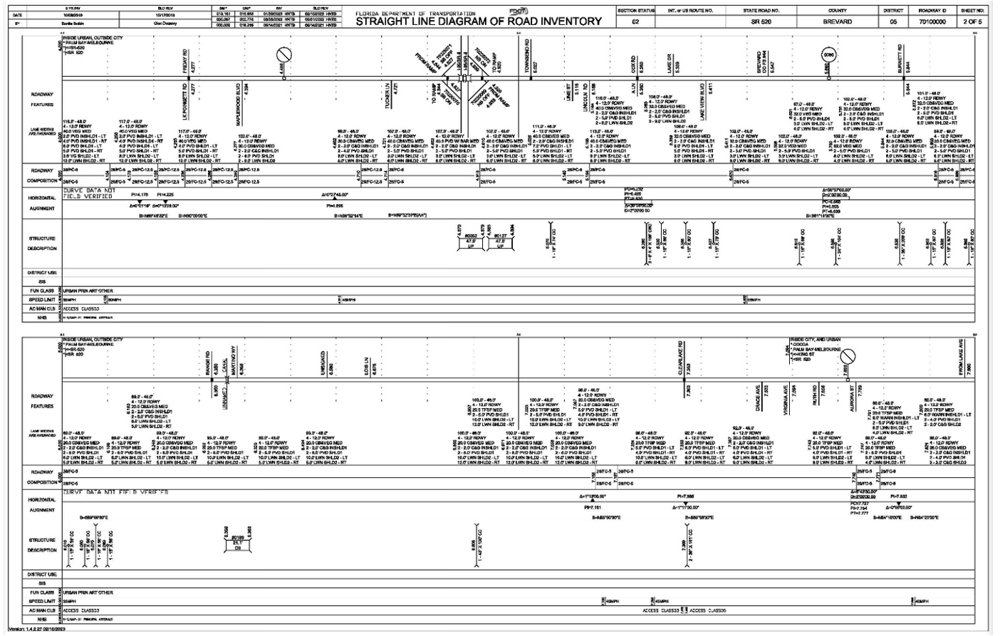
Figure 3-2 Straight Line Diagram Example

Step 3: Request Model Volumes

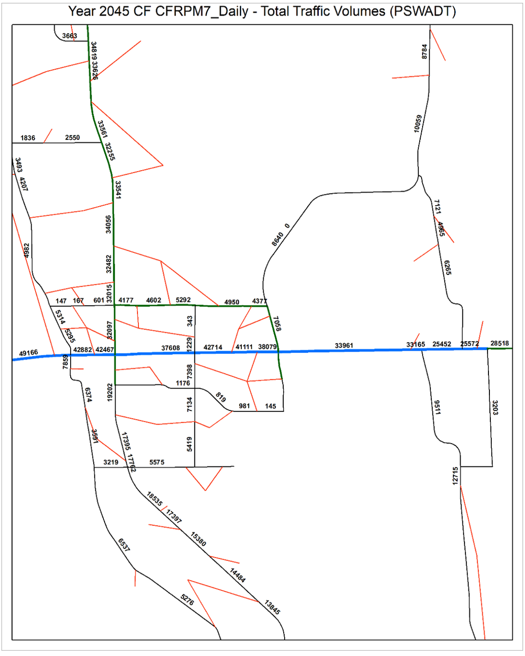
Request the modeling staff to provide adopted model volumes for both base year and future year for the project area. Convert the model data from PSWADT to AADT using MOCF if needed. Figure 3-3 shows an example of model volume plot displaying assigned traffic volume along the study corridor in Brevard County.

Step 4: Determine Existing Year AADT

Calculate average daily traffic volumes from short-term vehicle classification counts. Apply an appropriate Seasonal Factor to convert the ADT to AADT. No axle adjustment is needed if vehicle classification counts are collected. In this example, 48-hour classification counts were taken on August 23 and 24, 2022. The daily counts for the two days are 32,572 and 32,553. The corresponding Season Factor is 1.05. The Existing Year AADT is calculated as follows:

ADT=(32,572+32,553)/2=32,563

AADT=ADT×SF=32,563×1.05=34,191

AADT=34,000 (After applying rounding)

Step 5: Determine Design Traffic Characteristics

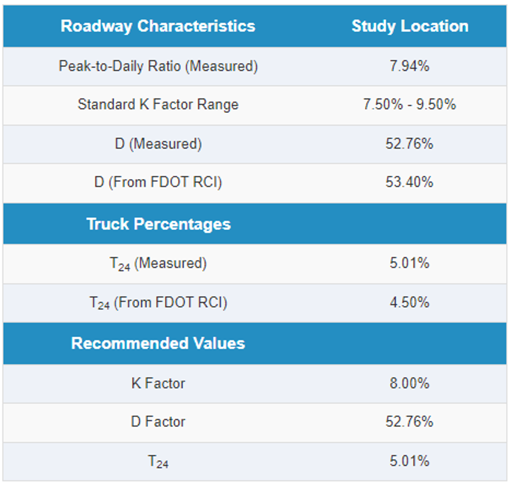
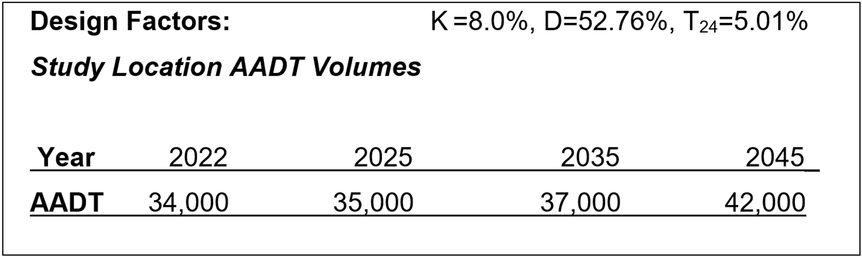
Develop design hour factors K, D, and T24 following the guidelines described in Chapter 2. The subject facility is a suburban arterial and the roadway context classification is Suburban Commercial (C3C). In this example, the measured Peak-to-Daily ratio was 7.94%, which is within the Standard K Range for the facility. The "D" value based on the short-term classification counts was 52.76% for the study location. The FDOT RCI database reported a D value of 53.40% for a FDOT Short-Term TMS site nearby. The measured daily truck factor (T24) from the classification count was 5.01%. The FDOT RCI database reported a daily truck factor of 4.50% for the same FDOT Site. Based on the comparison, the Standard K-Factor of 8.00%, the D Factor of 52.76%, and the daily truck factor (T24) of 5.01% are recommended, all based on field measured data at the site.

Table 3-1 Determine Design Hour Factors Example

Step 6: Develop Future Year Traffic Forecast

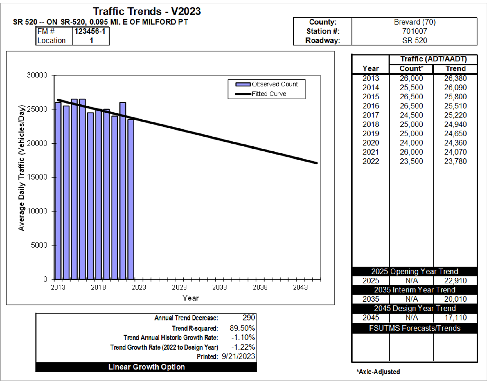
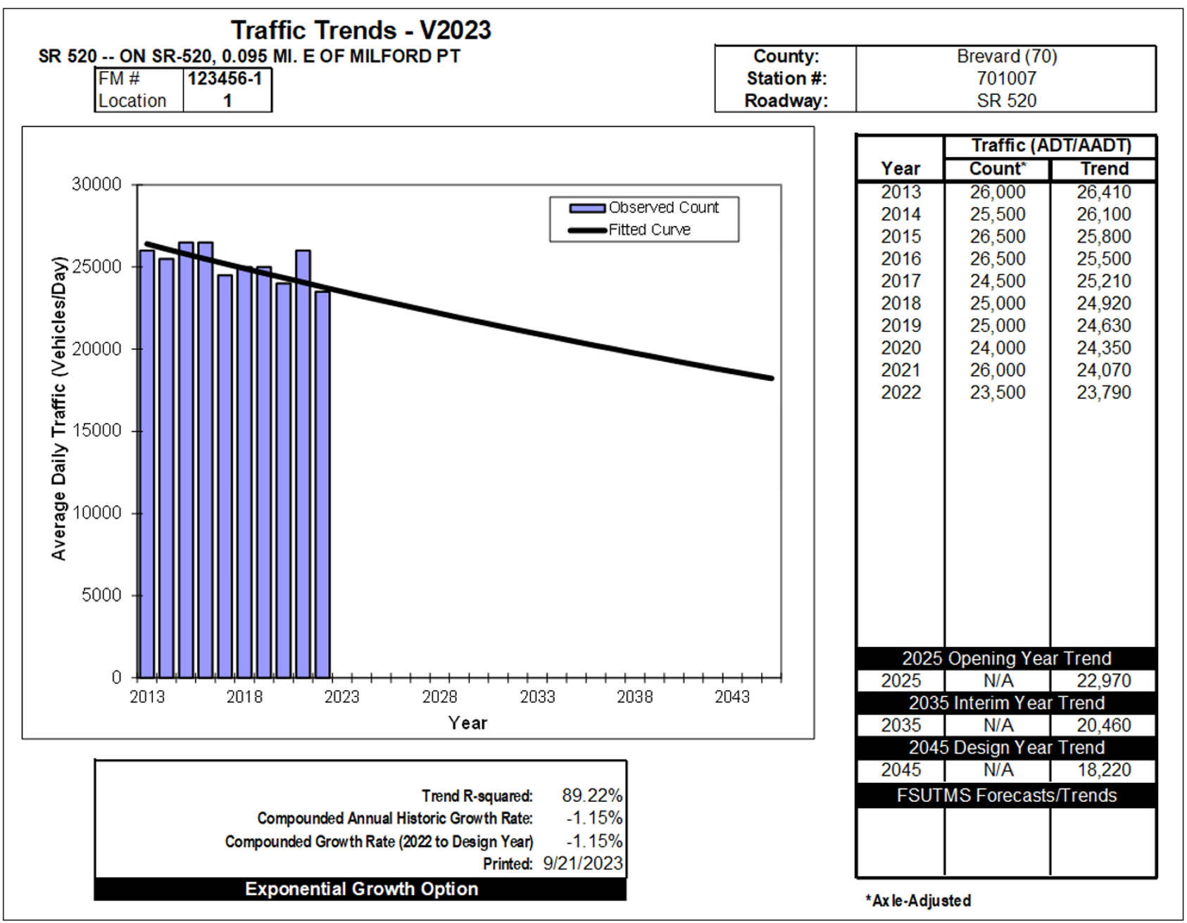
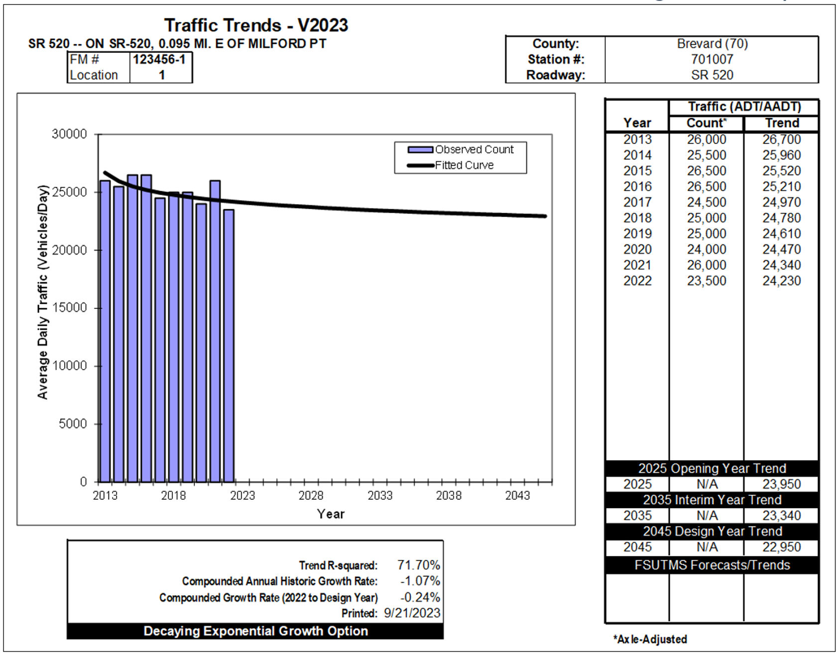
In the same example, historical AADT volumes are available at a Short-Term TMS site within the project limits. The AADT volumes for the past ten years from 2013 to 2022 are used for Trend Analysis. It should be noted that the reported AADT for 2020 is still used even though it is for the pandemic year. A careful evaluation of the 2020 AADT indicates that there are no significant differences in volumes between the adjacent years and the 2020 AADT generally follows the growth trend. Trend analysis was conducted first to determine the growth pattern and growth rate to be used for traffic forecasting. Figure 3-4, Figure 3-5, and Figure 3-6 show the trend analysis results using Linear Growth Option, Exponential Growth Option, and Decaying Exponential Growth Option, respectively. The R-Squared values for the three growth options are all higher than 70%, indicating a good fit in all cases. However, all three options show a negative growth. Thus, historical AADTs were not used for future travel demand forecasting.

Other sources of data were evaluated to calculate the growth rate. The growth rate calculated based on base year and future model data was 0.40%. In addition, Year 2022 population estimate and Year 2025 to 2045 population projections were obtained from the BEBR at University of Florida, and the population growth rate was determined to be 0.82%. Based on the comparison of growth rates obtained from various sources and in consultation with the FDOT, an annual growth rate of 0.60% was recommended to obtain the Opening Year 2025, Interim Year 2035 and Design Year 2045 projections for the study location.

With base year (2022) AADT of 34,000 and a growth rate of 0.60%, future year AADTs can be estimated using simple linear growth option as shown in Figure 3-7.

Step 7: Prepare Input Data for ESAL Calculation Spreadsheet

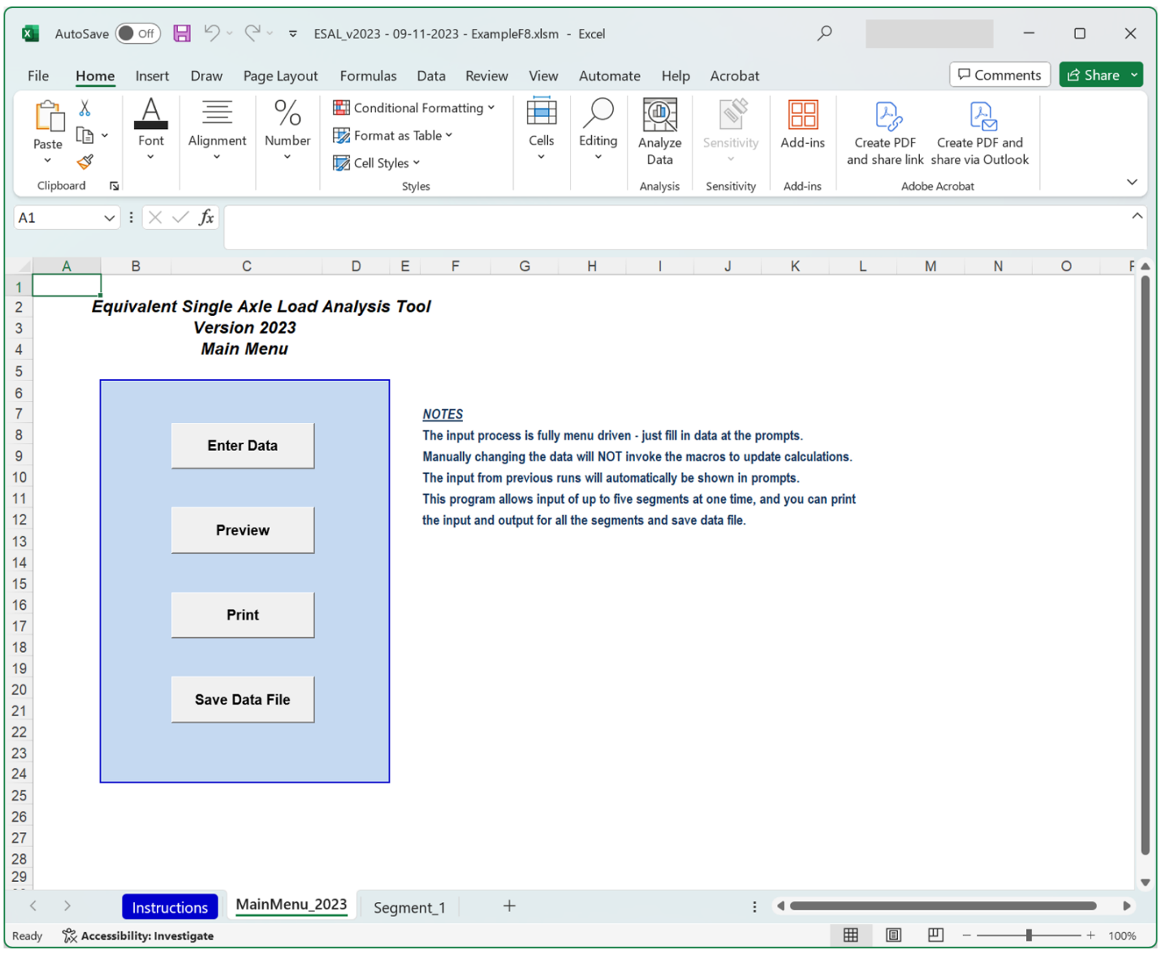
Open ESAL_V2023.XLSM. This Excel spreadsheet is a user-friendly menu/macro driven tool for input, calculation, and printing of ESALs. It can process up to five (5) roadway segments at the same time. Figure 3-8 shows the main menu of the ESAL Tool, Version 2023. The input process is fully menu driven. Enter the required information obtained from previous steps, and select the pavement type and Daily Directional Split, the spreadsheet will automatically calculate the required ESALs.

Example:

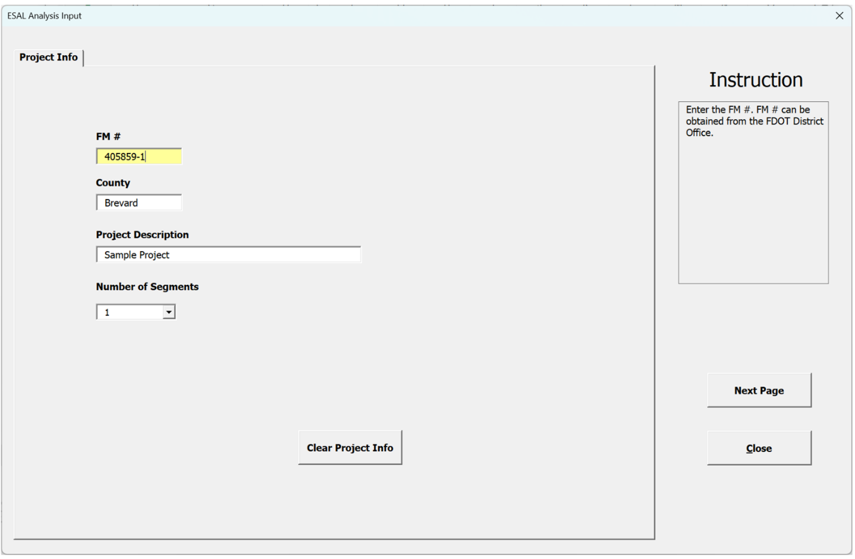
1. Enter project information. The project information includes FM number, project description, and number of segments. Number of segments is a required input. Click on the button "Clear Project Info" button to clear all the project information, including the data for the old roadway segment. The number of segments is set to 1 for this example. The Project Information input screen is shown in Figure 3-9.

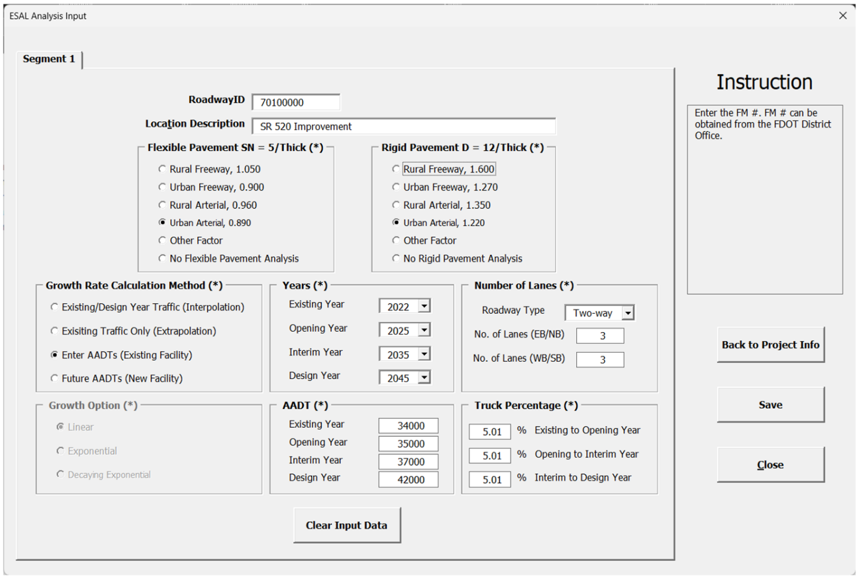
2. Enter roadway segment information for all segments, which may include Roadway ID, Location Description, Type of Roadway for Flexible Pavement, Type of Roadway for Rigid Pavement, Growth Rate Calculation Method, Years, Number of Lanes (by direction), Growth Option, AADT Volumes, Growth Rate, and Truck Percentages. If the new data for the segment is needed, click on the "Clear Input Data" button to clear the data for the segment. If the number of segments need to be changed, click on "Back to Project Info" button to go back to Project Info page, then change the number of segments and go to the next page to enter all information. Once the data for all segments is finished, click the "OK" button to complete the ESAL analysis. The roadway Segment Information input screen is shown in Figure 3-10.

3. Preview results: click the “Preview” button to show all the input and output for each roadway segment.

4. Print results: click the "Print” button to print out the input and output for all the roadway segments.

Step 8: Print Output Report from ESAL Calculation Spreadsheet

Print out the 18-KIP Report and prepare the transmittal memo. Have the designated traffic engineer review and sign the memo and 18-KIP Report. Figure 3-11 shows an example of the Output screens for the sample project.